Build Reports (SerialEM)

When building very large scale volumes it is useful to understand how the capture system is working. To facilitate this in SerialEM Nornir has the ability to produce reports for a volume or set of mosaics.

The current (2/27/14) report system provides the information overviewed below. Reports can be customized with python.

A full report for a subset of our mouse retinal connectom volume is visibile at http://connectomes.utah.edu/NornirExample/TEM/ImageReport.html/

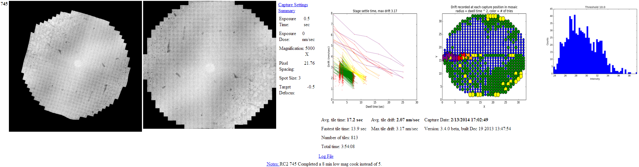
Output image summary: The image registered to the volume is to the left. The unregistered mosaic built from tiles is to the right.

Notes: If a notes.txt file was saved in the same directory as the .idoc file the raw text is injected at the bottom of the report. The raw notes may be accessed via the link.

Acquistion settings, speed and stage drift

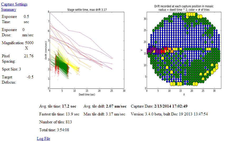
Settings: These are visible on the left and document the SerialEM and microscope settings used to capture the image. They are pulled from the .idoc file available by clicking the “Capture Settings Summary” link. Pixel spacing is in angstroms.

Drift: These figures show how long each individual tile had to sit before the tissue and stage drift rate slowed enough for SerialEM to capture an image. Drift rate is assessed during autofocus.

Points are color coded according to the number of focus attempts. SerialEM captures the image regardless after five attempts.

• Blue 1st autofocus attempt.

• Green 2nd autofocus attempt.

• Yellow 3rd autofocus attempt.

• Red 4th autofocus attempt.

• Purple 5th autofocus attempt.

This feedback is helpful in determining the effectiveness of stage settling mitigation strategies.

Statistics: Most of these fields are self explanatory. The following are the most useful for optimization:

• Fastest tile time indicates the best possible performance your scope is able to achieve during captures.

• Avg tile time indicates how far your scope falls from the fastest tile time. Subtract the average from the fastest time and multiple by the number of tiles to determine how much time could be gained with perfect optimization.

• Avg/Max drift can be multiplied by the exposure time and divided by the resoultion/pixel to measure what fraction of a pixels intensity is contributed by neighboring pixels. If the tile drifts a significant fraction of a pixel spacing during the exposure time the pixel will be blurry and one may be better off using a lower resolution and saving storage space and time.

Log File: The SerialEM log file contains the data required to quantize drift. The raw data can be accessed via the log file link.

Working with imperfect captures

Both electron and optical microscopy acquisitions can feature large empty regions. Featureless tiles are easily misregistered and discarding them saves storage and processing time. Empty tiles also throw off the default autocontrast settings for Nornir.

For the remaining examples feature the report below from a torn section. The report was generated with an older version but contains the relevant information.

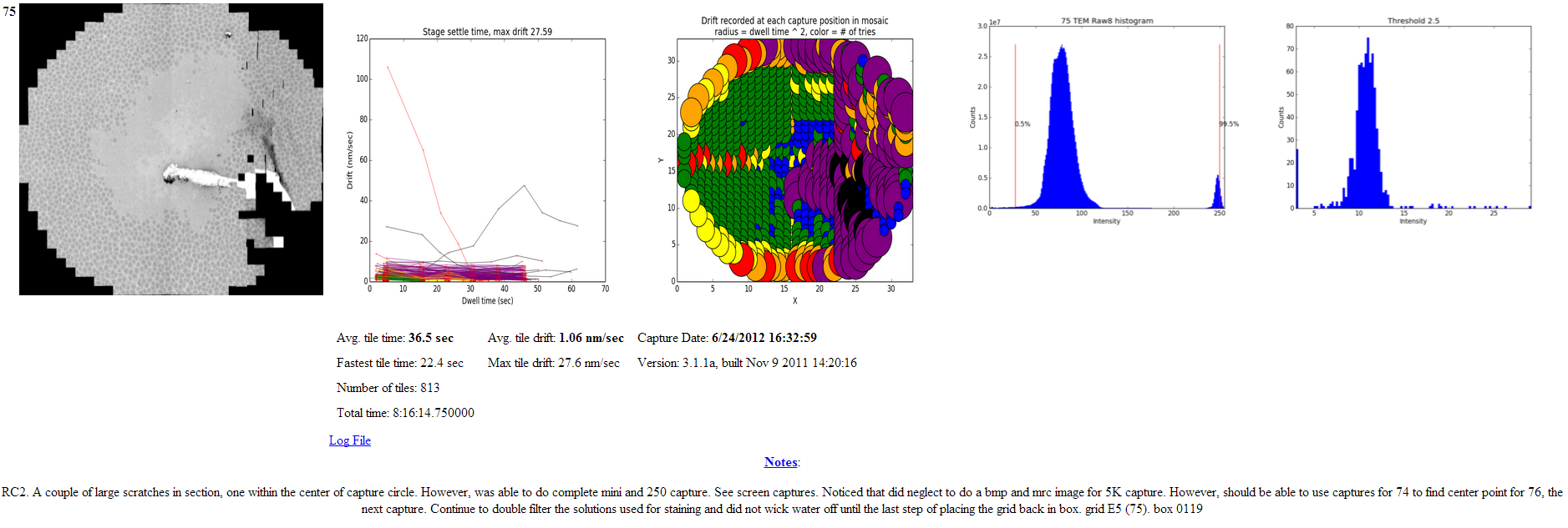
Note in the drift map how the region around the tear experienced predictable increases in tissue movement during capture.

Mark sections as damaged

A damaged section, even after repair, is almost always unsuitable to contribute to the slice-to-volume transformation series. These relevant section should be marked as damaged with the ‘’MarkSectionsDamaged’’ pipeline. The section will still participate in the volume, however any downstream sections will not use the damaged section to determine their volume position.

Remove featureless tiles

Nornir’s prune stage assigns a feature score to each tile based on the standard deviation of a small regions around the edge of each tile. The prune histogram suggests where the prune cutoff should be set to eliminate blank tiles with low prune scores.

The prune histogram indicates how each tile scored. The blank tiles can be seen clustered to the left with low scores. In this example I would first set a prune threshold of 5, rebuild and re-evaluate.

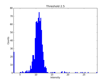
For this example I would suggest setting the max cutoff to 125 and not setting a low cutoff value.

Prune cutoffs are set with the SetPruneCutoff pipeline.

Adjust the contrast

Because of the tear we still have empty areas of high intensity and low interest. This produces the rightmost peak on the histogram. Folds can also occur which result in darker regions causing peaks to the left.

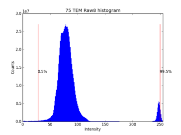
The histogram is recalculated after the prune threshold is changed. However it is often necessary to manually set a cutoff for autolevelling the histogram. The default behavior for the TEM scripts is to adjust Gamma so that the median intensity sits at 50%. This results in less contrast overall but preserves details in dense features such as synapses and gap junctions.

Contrast cutoffs are set with the SetContrast pipeline.

Optimizing Capture (SerialEM)

Comparing the two reports above it can be seen that the average tile time decreased from 36.6 to 17.2 seconds. While much of this is due to work Dave Mastronarde did to improve performance the operators have considerable control over capture speed.

A good image requires a long enough exposure to free the image from random noise and little tissue movement during exposure to preserve contrast. In capturing large volumes we must stabilize the image as fast as possible to capture as fast as possible while keeping the quality above a consistent standard. The first retinal connectome required about 341,000 captures. Saving a few seconds with optimization can save a project months of time.

Stage Drift

Stages require time to settle after a movement. SerialEM allows the operator to adjust the maximum amount of measured drift before an image is captured. Waiting for settling requires time and different mitigation strategies are available. Cooking at low or high magnifications can reduce the time for the tissue to cease movement when exposed to the electron beam. The diameter of the beam effects how much of the tissue surrounding the capture area is under strain. The range in capture time can be extreme. At 5000X the Marc lab can adjust spot size, beam diameter, and cooking stragies to observe a 16.5 sec/tile to 25 sec/tile range in performance.

We’ve found that a narrow beam diameter combined with a high-magnification cook does the best job of minimizing drift.

Image quality

The motivation to reduce drift is to preserving image contrast. One needs to ensure that the maximum drift is not moving a significant fraction of a pixel during the exposure time. The Marc lab uses a resolution of 2.176 nm/pixel. Our drift limit is 2.5 nm / sec. While we generally avoid the worst case some tiles may be blurred 50% with a neighboring pixel.

Reducing the drift limit increases capture time. The effects of high drift can also be hard to observe unless one uses the logs to ensure a high-drift tile is being examined.